Basic Layout

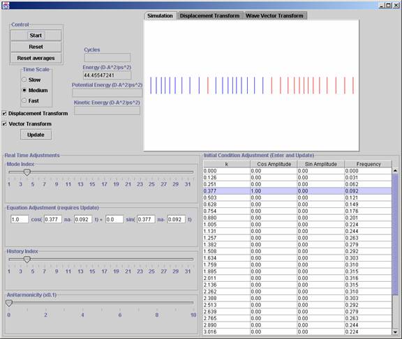
In the upper left hand corner you have the “Start”, “Reset” and “Reset averages” buttons. Only the former two do anything. The start button both starts and pauses the simulation. The reset button both pauses and resets positions to a t=0 state (note: values that dictate these initial conditions are taken from the settings set below, rather than the default)

Below that is a “Time Scale” selection box: this allows you to speed up or slow down the simulation. (note: time scaling too fast will result in decrease in calculation accuracy, and the simulation may become chaotic if such a decrease is significant)

Next there are 2 check boxes:

“Displacement Transform” toggles whether the simulation will perform the first Fourier transform on the displacements of the atoms. When turned on, the displacement transform windowpane will graph the wave components of the motion. If turned off, the windowpane will graph the displacements of the atoms.

“Vector Transform” toggles the second Fourier Transform. If on, the simulation will transform the change with respect to time of a particular value found in the first transform, displayed in the Wave Vector Transform windowpane. To select which value to monitor, use the History Index Slider. If off, it will simply display the logged history of the value’s change over time.

The “Update” button is basically a reset button, however it resets all conditions to current settings and then starts the simulation. Used for updating a change in settings.

To the right are the Meter Displays:

“Cycles” displays the number of cycles run, more or less the time of the system.

“[Total] Energy”, “Potential Energy”, and “Kinetic Energy” calculate and display the labeled value of the System of atoms. Note conservation of energy with constancy of Total Energy.

To the right of that are 3 tabbed windowpanes. Each windowpane displays different aspects of the simulation.

“Simulation” shows the atomic motion in the system, each “stick” representing one monatomic atom. The 2 Transform panes show the different Fourier Transforms of the simulation. The former transforming the displacement of the atoms, the latter transforming the wave vector derived from the former transform. These two transforms can be turned on and off using the checkboxes on the left.

Under the windowpanes is the “Equation Adjustment”. This allows you to change the starting conditions to a wave that would have these values. Input the values, press enter. In order to input multiple equations, one can use the “Mode Index Slider” to select another equation mode. There are 25 modes and they basically are an array of equations which you can traverse and input using the wave equation input.

The Bottom left is the “Real Time Adjustment” Section. These options can be changed and input while the program is running. The “Mode Index Slider” can show you which line of the table corresponds to the current equation adjustment input. The “Equation Adjustment” allows you to change the equation of the mode. (Note: this feature and the “Initial Condition Adjustment” table perform the same task).

“History Index” traverses the history view in the “Wave Vector Transform” Pane.

“Anharmonicity Slider” changes the coefficient of a cubic term in the harmonic potential. Setting this to a non-zero value will influence the wave by disrupting harmonicity.

Lastly, the “Initial Condition Adjustment” table. It is basically a table form of the equation input area under the Window Panes. Input values and press the Update button.